OneHotEncoder

Hopefully, by the end of this, you will understand what scikit-learn’s OneHotEncoder does and why, how to interpret linear regression coefficients from OneHotEncoder, why you should drop one column / category when you use OneHotEncoder, and how to pick which one!

I’m going to use a slightly ridiculous regression example to illustrate these points, but stick with me and it will be worth it in the end!

What data are we using?

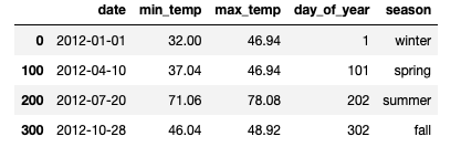
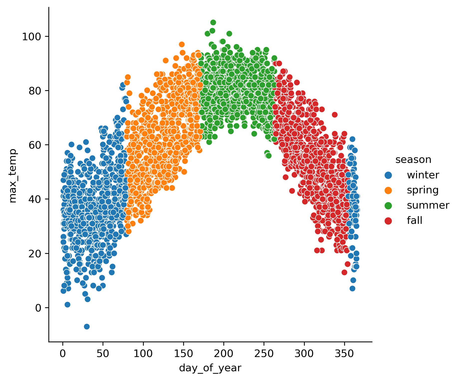
Let’s use this simple dataset, with temperature data from a weather station in Chicago (more on that in a separate post), where they experience four different seasons. Using the datetime stamp from the weather station measurements, I created two features: day_of_year and season. Let’s plot max temperatures across the year, with data points labelled by season. Here’s a peek at the data we’re using.

# Use pandas to work with DataFrame
import pandas as pd

# read in csv
df_temp = pd.read_csv('data/temp_data.csv')
df_temp.iloc[[0,100,200,300]]

# nice simple plots
import seaborn as sns

sns.relplot(x='day_of_year', y='max_temp', hue="season", data=df_temp);

What happens if you use a categorical variable as a predictor?

Let’s assume that I want to predict daily max_temp using that categorical season label. We could try using Linear Regression!

from sklearn.linear_model import LinearRegression

lr = LinearRegression()
lr.fit(df_temp[['season']], df_temp[['max_temp']])

---------------------------------------------------------------------------
ValueError                                Traceback (most recent call last)
<ipython-input-4-60806040f9d7> in <module>
      2 
      3 lr = LinearRegression()
----> 4 lr.fit(df_temp[['season']], df_temp[['max_temp']])

/opt/anaconda3/envs/learn-env/lib/python3.8/site-packages/sklearn/linear_model/_base.py in fit(self, X, y, sample_weight)
    503 
    504         n_jobs_ = self.n_jobs
--> 505         X, y = self._validate_data(X, y, accept_sparse=['csr', 'csc', 'coo'],
    506                                    y_numeric=True, multi_output=True)
    507 


** A BUNCH MORE ERRORS **
 

ValueError: could not convert string to float: 'winter'

Unfortunately, it fails when you try to use a string variable as a predictor. Apparently, LinearRegression only wants to do math with numbers. But, we know that season is probably related to max_temp. How can we convert the season labels to numbers that LinearRegression can understand?

Is season an ordinal variable?

Couldn’t we just code season as an ordinal variable? What if we assign numbers to each season based on the order it occurs in the year (“winter” = 1, “spring” = 2, etc.)? Well, that doesn’t quite work here. One issue is that winter comes before spring, but also after fall. So should we label that second winter as ‘5’? Perhaps more importantly, using ordinal variables in linear regression would effectively rank the different categories, such that 3 would be more than 2 but less than 4. But, is summer more season-y than spring and less season-y than fall? Nope.

OneHotEncoder makes a separate variable for each category

This is where one-hot encoding comes into play. OneHotEncoder converts categorical variables to multiple columns with numeric values. Each column contains 0’s and 1’s, with 1 indicating when the category is present or true, and 0 when it is absent or false.

ohe = OneHotEncoder(drop=None, sparse=False)
season_trans = ohe.fit_transform(df_temp[['season']])
season_df = pd.DataFrame(season_trans, columns=ohe.get_feature_names())
pd.concat([df_temp, season_df], axis=1).iloc[[0,100,200,300]]

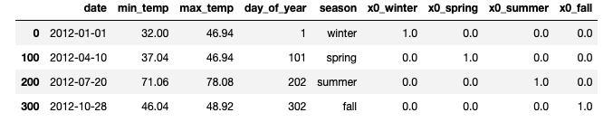
These separate columns can then be entered into multiple regression, and combined can capture how your categorical predictor relates to your target variable.

Why does OneHotEncoder drop a column by default?

One thing about OneHotEncoder that can be confusing is why we’re advised to drop one category when using linear regression (at least without regularization / penalty). If we consider the information provided by each column, it turns out that the final column provides no additional information. In this case, if the columns for ‘spring’, ‘summer’, and ‘fall’ are all 0’s, then we know the day didn’t belong to any of those seasons. Therefore, that day must belong to ‘winter’. We don’t need to see a 1 in the ‘winter’ column to know that. (We might need to wait for another blog post to find out what happens if you do use all four columns.)

Let’s try again to predict max_temp with three of the one-hot encoded variables, and see what the LinearRegression can tell us.

y = df_temp['max_temp']
X = season_df[['x0_fall', 'x0_spring', 'x0_summer']]
lr = LinearRegression()
lr.fit(X, y)

LinearRegression()

The model now runs, since we’re using columns of numbers. Let’s see if we can figure out what the output means. One cool thing about linear regression is that you should be able to interpret its coefficients in a very straightforward way.

Interpret linear regression coefficients by plugging them into the formula for a line

I learned the equation for a straight line long ago.

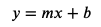
where ‘m’ is the slope of the line, and ‘b’ (also called the intercept) is the value when x is 0.

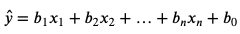
In linear regression, the letters have changed, but the idea is the same.

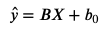
The capital B and X are matrices that each contain multiple values. The multiple b values (known as coefficients) correspond to the slopes for each of the x variables. The B0 value is the intercept.

So, let’s see what the linear regression model tells us about the relationship between maximum temperature and each of the seasons. In order to do that, let’s get the intercept and coefficients from our LinearRegression, and start putting numbers into that formula for our line.

print("Intercept: ", lr.intercept_)
print("Coefficients: ", lr.coef_)

Intercept:  36.85649484536082
Coefficients:  [25.35550976 42.67644763 16.83120771]

The three coefficients correspond to the three variables we entered, in the order that we entered them. But, what about ‘winter’? How do we figure out our predicted temperature for winter? Well, remember that ‘winter’ occurs when all of the other columns have values of 0. So, the equation for that line becomes:

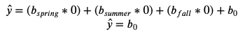
LinearRegression gave us 36.85649484536082 for b0 (the intercept), so that’s our predicted maximum temperature for each winter day.

Is that a good guess? Actually, it’s the best guess that we could make! If the only thing we know is that the day occurred during the winter, the guess that would would minimize the sum of squared errors is the mean of max_temp for winter days. And what is the mean for winter days? You guessed it…

criteria = (df_temp['season'] == 'winter')
print("Mean winter: ", df_temp['max_temp'][criteria].mean() )
print("Intercept: ", lr.intercept_)

Mean winter:  36.85649484536083
Intercept:  36.85649484536082

Well, that’s pretty cool! We were able to get a prediction for maximum temperature of winter days without giving LinearRegression a column of predictors for winter. The B0 intercept is the mean of the dropped category (more specifically, the estimate when all other variables in the model equal 0).

Now, what about spring? Let’s take a look at the formula for our line. But this time, let’s insert a 1 as the variable for spring.

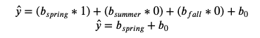
So, to get the prediction for spring, we need add the coefficient for the spring column to the b0 intercept value.

criteria = (df_temp['season'] == 'spring')
print("Mean spring: ", df_temp['max_temp'][criteria].mean() )
print("Spring: ", lr.intercept_ + lr.coef_[0])

Mean spring:  62.21200460829493
Spring:  62.21200460829499

So, the coefficient for each column represents the difference between that category and the left out category. More specifically, for each unit change in x, y will change by b units, above and beyond the intercept value).

In fact, you can predict the mean of each season this way:

Winter:

Spring:

Summer: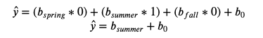

Fall: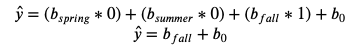

order = ['winter', 'spring', 'summer', 'fall']
df_temp.groupby('season')['max_temp'].mean()[order]

season
winter    36.856495
spring    62.212005
summer    79.532942
fall      53.687703
Name: max_temp, dtype: float64

print("Winter: ", lr.intercept_)
print("Spring: ", lr.intercept_ + lr.coef_[0])
print("Summer: ", lr.intercept_ + lr.coef_[1])
print("Fall:   ", lr.intercept_ + lr.coef_[2])

Winter:  36.856494845360814
Spring:  62.21200460829499
Summer:  79.53294247787608
Fall:    53.6877025527192

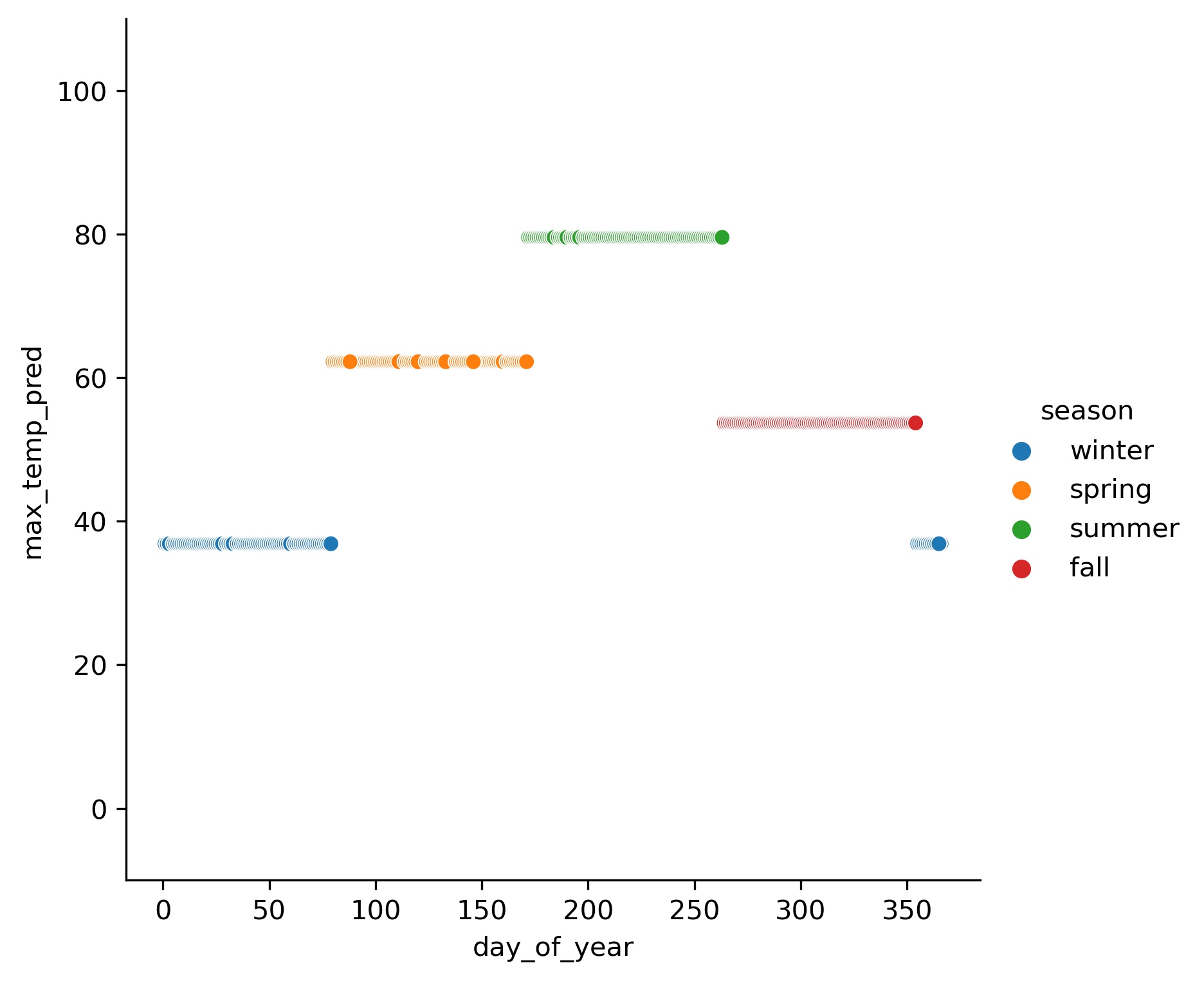
df_temp['max_temp_pred'] = lr.predict(X)

h = sns.relplot(x='day_of_year', y='max_temp_pred', hue="season", data=df_temp)
h.set(ylim=(-10, 110));

Hopefully, this helps you understand what OneHotEncoder does, and how you can use and interpret it in a linear regression model!