If you’re just starting to work with time series analysis, you may be coming across terms like autocorrelation function (ACF) and partial autocorrelation function (PACF).
To go from “confused” to “comprende”, let’s dissect these terms to find out what they really mean.
What’s the difference between a correlation and autocorrelation?
By now, you’re very familiar with the concept of a correlation, which calculates the linear relationship between two variables. Well, an autocorrelation show the relationship between a variable and itself, at some point in the past.
That’s all well and good, but why should we care our time series is autocorrelated? Just like an author can write a biography about another person, a variable can tell a story about another variable with which it is correlated. Similarly, a time series with autocorrelation can write an autobiography about itself, providing some insight to that time series that we might not have had otherwise.
Where this gets really interesting (and where the “autobiography” analogy breaks down a bit) is when we’re interested in predicting the future! With two correlated variables, it may be possible to use values from one variable to predict unknown values of the other variable. Similarly, if a time series is autocorrelated with itself in the past, then we might be able to use known past values of the time series to predict its future!
What does an autocorrelation look like?
For this demonstration, we’re going to work with data from Google Trends. Specifically, our google_trends data frame has a diet column containing monthly estimates of “interest over time” for the search term “diet” from 2004 through 2018.
google_trends.plot(figsize=(12,6))
plt.xlabel('Year', fontsize=14);
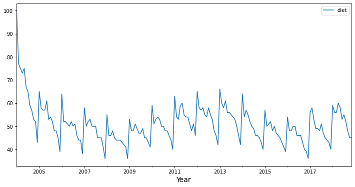
Visually, you can recognize patterns in these data. We can see a yearly seasonality, with a spike in interest in “diet” near the beginning of the year, with a gradual decline in interest throughout the rest of the year. Given that repeated pattern, we can probably use information about the past time series values to predict what will happen in the future.
Let’s add some columns that shift our time series in time. That allows us to capture past “lags” and compare them against the present (unshifted time series). The make_lag_dataframe() function uses the .shift() method to slide the original time series by some lag, and then returns a new data frame with the original and shifted time series.
def make_lag_dataframe(ts_df, n_lags):
    my_ts_df = ts_df.copy()
    basename = list(my_ts_df.columns)[0]
    col_names = [basename + '_tminus_0']
    for lag in range(1,n_lags+1):
        my_ts_df = pd.concat([my_ts_df, ts_df.shift(periods=lag)], axis=1)
        col_names.append(basename + '_tminus_' + str(lag))
    my_ts_df.columns = col_names
    return my_ts_df
Make the lag time series
Let’s shift the time series, so we can correlate past values with the original time series. Notice that we get some NaNs at the top of the shifted columns, because those time points would have occurred in 2003, and we don’t have access to data from 2003.
diet_df = make_lag_dataframe(google_trends, 20)
diet_df.head(10)
| diet_tminus_0 | diet_tminus_1 | diet_tminus_2 | diet_tminus_3 | diet_tminus_4 | diet_tminus_5 | diet_tminus_6 | diet_tminus_7 | diet_tminus_8 | diet_tminus_9 | ... | diet_tminus_11 | diet_tminus_12 | diet_tminus_13 | diet_tminus_14 | diet_tminus_15 | diet_tminus_16 | diet_tminus_17 | diet_tminus_18 | diet_tminus_19 | diet_tminus_20 | |
|---|---|---|---|---|---|---|---|---|---|---|---|---|---|---|---|---|---|---|---|---|---|
| month | |||||||||||||||||||||
| 2004-01-01 | 100 | NaN | NaN | NaN | NaN | NaN | NaN | NaN | NaN | NaN | ... | NaN | NaN | NaN | NaN | NaN | NaN | NaN | NaN | NaN | NaN |
| 2004-02-01 | 77 | 100.0 | NaN | NaN | NaN | NaN | NaN | NaN | NaN | NaN | ... | NaN | NaN | NaN | NaN | NaN | NaN | NaN | NaN | NaN | NaN |
| 2004-03-01 | 75 | 77.0 | 100.0 | NaN | NaN | NaN | NaN | NaN | NaN | NaN | ... | NaN | NaN | NaN | NaN | NaN | NaN | NaN | NaN | NaN | NaN |
| 2004-04-01 | 73 | 75.0 | 77.0 | 100.0 | NaN | NaN | NaN | NaN | NaN | NaN | ... | NaN | NaN | NaN | NaN | NaN | NaN | NaN | NaN | NaN | NaN |
| 2004-05-01 | 75 | 73.0 | 75.0 | 77.0 | 100.0 | NaN | NaN | NaN | NaN | NaN | ... | NaN | NaN | NaN | NaN | NaN | NaN | NaN | NaN | NaN | NaN |
| 2004-06-01 | 67 | 75.0 | 73.0 | 75.0 | 77.0 | 100.0 | NaN | NaN | NaN | NaN | ... | NaN | NaN | NaN | NaN | NaN | NaN | NaN | NaN | NaN | NaN |
| 2004-07-01 | 65 | 67.0 | 75.0 | 73.0 | 75.0 | 77.0 | 100.0 | NaN | NaN | NaN | ... | NaN | NaN | NaN | NaN | NaN | NaN | NaN | NaN | NaN | NaN |
| 2004-08-01 | 59 | 65.0 | 67.0 | 75.0 | 73.0 | 75.0 | 77.0 | 100.0 | NaN | NaN | ... | NaN | NaN | NaN | NaN | NaN | NaN | NaN | NaN | NaN | NaN |
| 2004-09-01 | 57 | 59.0 | 65.0 | 67.0 | 75.0 | 73.0 | 75.0 | 77.0 | 100.0 | NaN | ... | NaN | NaN | NaN | NaN | NaN | NaN | NaN | NaN | NaN | NaN |
| 2004-10-01 | 53 | 57.0 | 59.0 | 65.0 | 67.0 | 75.0 | 73.0 | 75.0 | 77.0 | 100.0 | ... | NaN | NaN | NaN | NaN | NaN | NaN | NaN | NaN | NaN | NaN |
10 rows × 21 columns
Plot the lag time series
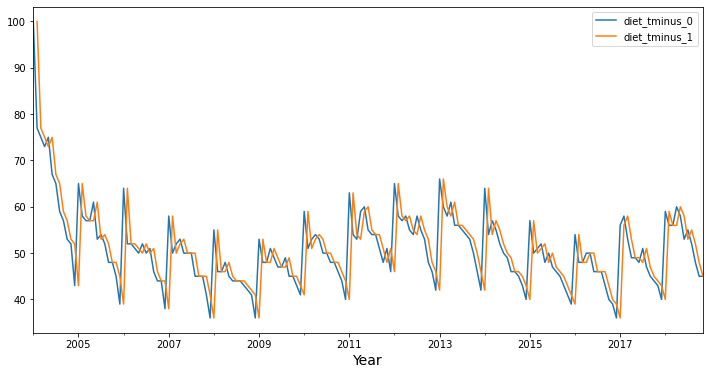
Now, let’s see what a lag 1 autocorrelation looks like with these data. Again, it looks visually like the lag 1 time series diet_tminus_1 (in orange) might correlate with the original time series (in blue), and consequently, we might be able to “predict” the original time series using the lag 1 time series (from one month in the past)!
diet_df[['diet_tminus_0', 'diet_tminus_1']].plot(figsize=(12,6))
plt.xlabel('Year', fontsize=14);
Predict original time series from the past time series
Let’s see if we can run a linear regression model to see how much our original time series is explained by the “lag 1” values (from one month in the past).
import statsmodels.api as sm
lag1_df = diet_df[['diet_tminus_0', 'diet_tminus_1']].dropna()
y = lag1_df['diet_tminus_0']
X = lag1_df[['diet_tminus_1']]
sm.OLS(y, sm.add_constant(X)).fit().summary()
| Dep. Variable: | diet_tminus_0 | R-squared: | 0.390 |
|---|---|---|---|
| Model: | OLS | Adj. R-squared: | 0.387 |
| Method: | Least Squares | F-statistic: | 112.7 |
| Date: | Sun, 01 May 2022 | Prob (F-statistic): | 1.15e-20 |
| Time: | 17:12:29 | Log-Likelihood: | -564.41 |
| No. Observations: | 178 | AIC: | 1133. |
| Df Residuals: | 176 | BIC: | 1139. |
| Df Model: | 1 | ||
| Covariance Type: | nonrobust |
| coef | std err | t | P>|t| | [0.025 | 0.975] | |
|---|---|---|---|---|---|---|
| const | 22.1608 | 2.730 | 8.118 | 0.000 | 16.774 | 27.548 |
| diet_tminus_1 | 0.5601 | 0.053 | 10.618 | 0.000 | 0.456 | 0.664 |
| Omnibus: | 59.848 | Durbin-Watson: | 2.327 |
|---|---|---|---|
| Prob(Omnibus): | 0.000 | Jarque-Bera (JB): | 125.079 |
| Skew: | 1.570 | Prob(JB): | 6.91e-28 |
| Kurtosis: | 5.647 | Cond. No. | 325. |
Yup! Almost 40% of the variance in the original timeseries can be explained by the time series values from one month before! Importantly, the regression coefficient for diet_minus_1 is 0.56, which is significanlty different from zero.
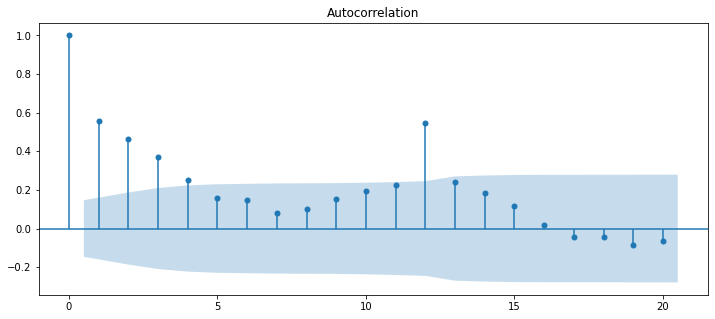
This where the autocorrelation function (ACF) comes in. Rather than making multiple lagged time series and then conducting linear regression on each of them, the ACF does all of those fun steps for you.
Plot the ACF graph
First, let’s see what is output by plot_acf in the statsmodels package.
from matplotlib.pylab import rcParams
rcParams['figure.figsize'] = 12, 5

from statsmodels.graphics.tsaplots import plot_acf
plot_acf(diet_df['diet_tminus_0'], lags=20);
Now, let’s compare those ACF parameters to the parameters from the linear regression. The function below will take the dataframe we created earlier (which contains the original time series and lagged time series columns), runs the OLS linear regression for a specific lag, and returns the parameter estimate relating that lag to the original time series. Then we can compare those parameter estimates to the values returned by the acf function built into statsmodels.
def full_param(df, lag):
    my_lag_df = pd.DataFrame()
    my_lag_df['y'] = df.iloc[:, 0]
    my_lag_df['X'] = df.iloc[:, lag]
    my_lag_df.dropna(inplace=True)
    par = sm.OLS(
        my_lag_df['y'], sm.add_constant(
        my_lag_df['X']  )
        ).fit().params[-1]
    return par
comp_df = pd.DataFrame()

from statsmodels.tsa.stattools import acf

comp_df['acf'] = acf(diet_df['diet_tminus_0'], nlags=20)
comp_df['fullregress'] = [full_param(diet_df, f) for f in range(0, 20+1)]

print(comp_df)
             acf  fullregress
    0   1.000000     1.000000
    1   0.558303     0.560142
    2   0.462154     0.465421
    3   0.367907     0.371177
    4   0.251550     0.254133
    5   0.157250     0.159263
    6   0.147585     0.149495
    7   0.082802     0.083963
    8   0.101360     0.102652
    9   0.151172     0.153270
    10  0.195190     0.198175
    11  0.227415     0.231661
    12  0.547641     0.568226
    13  0.238420     0.248687
    14  0.183618     0.192926
    15  0.115117     0.122045
    16  0.019305     0.021619
    17 -0.042552    -0.043581
    18 -0.043382    -0.044098
    19 -0.087285    -0.090209
    20 -0.064923    -0.066328
So, in essence, the autocorrelation function (acf) returns the set of parameter estimates (betas) that describe how each lagged timeseries (from the past) predicts the original time series.
NB: I believe that the reason these values are not precisely the same has something to do with how acf in the statsmodels library computes the mean and variance (using the full time series, before dropping NaNs). However, my goal for this blog post is to increase conceptual understanding of these topics, and a full investigation and discussion of this relatively minor difference is outside of its scope!
So, what is the partial autocorrelation function (PACF)?
If the autocorrelation is like an autobiography, does that mean that a partial autocorrelation is like an unfinished autobiography? Well, sort of…
Imagine that an author wrote their autobiography when they were 20, but then every year they wrote an additional chapter describing what has changed since their last update. The most recent chapter wouldn’t describe the author’s entire life, but instead would only describe the changes attributable to the most recent year.
Similarly, the partial autocorrelation describes only the change attributable to lag n above and beyond the contributions of previous lags. For example, a partial autocorrelation of lag 3 shows the increment in autocorrelation explained by lag 3 after removing (or partialling) the contributions of lag 2 and lag 1.
from statsmodels.graphics.tsaplots import plot_pacf
from matplotlib.pylab import rcParams

rcParams['figure.figsize'] = 14, 5

plot_pacf(diet_df['diet_tminus_0'], lags=20);
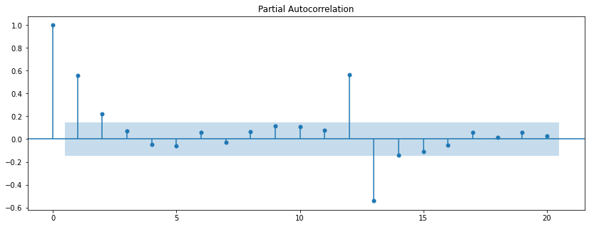
The distinction between “autocorrelation” and “partial autocorrelation” is essentially the same as the distinction between “correlation” and “partial correlation”. The partial correlation describes the relationship between two variables after removing the contribution of one or more other variables. The partial autocorrelation describes the relationship between the original time series and lag n time series after modeling the contributions of all time series for lags less than n.
Consequently, we can demonstrate partial autocorrelation in the context of a multiple regression. The function below computes a multiple regression to predict the original time series with each lag up to lag n, and then outputs the beta weight for the incremental (additional) contribution of lag n with all of the previous lags in the multiple regression model. Then we can compare those outputs to the pacf function from statsmodels.
def partial_param(df, n_lags):
    # lag 0 is the time series predicted by itself
    if n_lags == 0 :
        my_lag_df = df.iloc[:, 0].copy()
        y = my_lag_df
        X = my_lag_df
    else:
        my_lag_df = df.iloc[:, 0:n_lags+1].copy() # grab all columns up to and including 'n_lags'
        my_lag_df.dropna(inplace=True)
        y = my_lag_df.iloc[:, 0] # y is the original time series
        X = my_lag_df.iloc[:, 1:n_lags+1] # the X matrix is all columns from lag 1 through lag n_lags

    par = sm.OLS(
        y, sm.add_constant(
        X
        )).fit().params[-1]  # the last beta weight belongs to the last lag

    return par
from statsmodels.tsa.stattools import pacf

# pacf using 'ols' method only for illustrative purposes (to compare to sm.OLS)
comp_df['pacf'] = pacf(diet_df['diet_tminus_0'], nlags=20, method='ols')
comp_df['partialregress'] = [partial_param(diet_df, f) for f in range(0, 20+1)]

display(comp_df)
The last two columns give us the values from statsmodels pacf function and the beta weights from set of the multiple regression models we ran.
| acf | fullregress | pacf | partialregress | |
|---|---|---|---|---|
| 0 | 1.000000 | 1.000000 | 1.000000 | 1.000000 |
| 1 | 0.558303 | 0.560142 | 0.560142 | 0.560142 |
| 2 | 0.462154 | 0.465421 | 0.243824 | 0.243824 |
| 3 | 0.367907 | 0.371177 | 0.100474 | 0.100474 |
| 4 | 0.251550 | 0.254133 | -0.019043 | -0.019043 |
| 5 | 0.157250 | 0.159263 | -0.011044 | -0.011044 |
| 6 | 0.147585 | 0.149495 | 0.098490 | 0.098490 |
| 7 | 0.082802 | 0.083963 | -0.003919 | -0.003919 |
| 8 | 0.101360 | 0.102652 | 0.073544 | 0.073544 |
| 9 | 0.151172 | 0.153270 | 0.134398 | 0.134398 |
| 10 | 0.195190 | 0.198175 | 0.125446 | 0.125446 |
| 11 | 0.227415 | 0.231661 | 0.079914 | 0.079914 |
| 12 | 0.547641 | 0.568226 | 0.618342 | 0.618342 |
| 13 | 0.238420 | 0.248687 | -0.594229 | -0.594229 |
| 14 | 0.183618 | 0.192926 | -0.133914 | -0.133914 |
| 15 | 0.115117 | 0.122045 | -0.194105 | -0.194105 |
| 16 | 0.019305 | 0.021619 | -0.074346 | -0.074346 |
| 17 | -0.042552 | -0.043581 | -0.085653 | -0.085653 |
| 18 | -0.043382 | -0.044098 | -0.046873 | -0.046873 |
| 19 | -0.087285 | -0.090209 | 0.007411 | 0.007411 |
| 20 | -0.064923 | -0.066328 | 0.045361 | 0.045361 |
So, we can see that the partial autocorrelation function (pacf) returns the set of parameter estimates (betas) capturing the unique contribution of each lagged timeseries after removing the contributions from time series with lower order lag.
Bringing it back together
So, in the end, autocorrelation and partial autocorrelation are essentially the same as your old friends correlation and partial correlation. The main difference is that autocorrelation describes a correlation of the original time series with a version of itself from the past.
By creating shifted versions of the time series and using them to predict the original version in a regression framework, we saw that the autocorrelation function (ACF) was basically the same as the beta weights from a set of simple regression models, and the partial autocorrelation function (PACF) was the same as beta weights from a set of multiple regression models.
The real power in the concepts of ACF and PACF comes from the possibility that the relationships with past values of the time series might predict its future values.
To unleash that power, take these concepts and start working with SARIMAX models!